Supplementary Figure 2
Nils Eling and Nicolas Damond
2020-11-18
Last updated: 2020-11-18
Checks: 7 0
Knit directory: cytomapper_publication/
This reproducible R Markdown analysis was created with workflowr (version 1.6.2). The Checks tab describes the reproducibility checks that were applied when the results were created. The Past versions tab lists the development history.
Great! Since the R Markdown file has been committed to the Git repository, you know the exact version of the code that produced these results.
Great job! The global environment was empty. Objects defined in the global environment can affect the analysis in your R Markdown file in unknown ways. For reproduciblity it’s best to always run the code in an empty environment.
The command set.seed(20200602) was run prior to running the code in the R Markdown file. Setting a seed ensures that any results that rely on randomness, e.g. subsampling or permutations, are reproducible.
Great job! Recording the operating system, R version, and package versions is critical for reproducibility.
Nice! There were no cached chunks for this analysis, so you can be confident that you successfully produced the results during this run.
Great job! Using relative paths to the files within your workflowr project makes it easier to run your code on other machines.
Great! You are using Git for version control. Tracking code development and connecting the code version to the results is critical for reproducibility.
The results in this page were generated with repository version 6ccdd51. See the Past versions tab to see a history of the changes made to the R Markdown and HTML files.
Note that you need to be careful to ensure that all relevant files for the analysis have been committed to Git prior to generating the results (you can use wflow_publish or wflow_git_commit). workflowr only checks the R Markdown file, but you know if there are other scripts or data files that it depends on. Below is the status of the Git repository when the results were generated:
Ignored files:
    Ignored:    .Rproj.user/
    Ignored:    data/PancreasData/pancreas_images.rds
    Ignored:    data/PancreasData/pancreas_masks.rds
    Ignored:    data/PancreasData/pancreas_sce.rds

Unstaged changes:
    Modified:   analysis/04-Figure_1.Rmd
Note that any generated files, e.g. HTML, png, CSS, etc., are not included in this status report because it is ok for generated content to have uncommitted changes.
These are the previous versions of the repository in which changes were made to the R Markdown (analysis/04-Figure_S2.Rmd) and HTML (docs/04-Figure_S2.html) files. If you’ve configured a remote Git repository (see ?wflow_git_remote), click on the hyperlinks in the table below to view the files as they were in that past version.
| File | Version | Author | Date | Message |
|---|---|---|---|---|
| Rmd | 96b285d | Nils Eling | 2020-11-18 | Set correct figure paths |
| Rmd | 08f5f0d | Nils Eling | 2020-11-18 | Split figures into main and supplements |
This script reproduces the analysis performed in Supplementary Figure 2. Here, we will load the libraries and data for this figure:
library(cytomapper)
library(dplyr)

sce <- readRDS("data/PancreasData/pancreas_sce.rds")
images <- readRDS("data/PancreasData/pancreas_images.rds")
In line with Supplementary Figure 1, we will now order the images based on the mean intensity of all PIN positive pixels.
PIN_mean <- unlist(lapply(images,
                   function(x){
                     cur_x <- x[,,"PIN"]
                     mean(cur_x[cur_x > 0])
                   }))
Here, we will visualize the marker pro-insulin (PIN) across all images. Due to the progressive decline in beta cell function, we expect PIN expression to be reduced in Long-Duration patients. However, a similar analysis can be performed to visually detect image-to-image irregularities in background stain.
We will normalize across all images to keep the differences in staining intensity between images intact.
# Specify the image order
cur_order <- order(PIN_mean, decreasing = TRUE)

# Collect metadata for images
cur_meta <- as_tibble(colData(sce)) %>%
  group_by(ImageNumber) %>%
  summarise_at(vars("ImageName", "ImageFullName", "stage"), unique) %>%
  mutate(ImageFullName = gsub(".tiff", "", ImageFullName)) %>%
  as.data.frame()

rownames(cur_meta) <- cur_meta$ImageFullName
cur_meta <- cur_meta[names(PIN_mean)[cur_order],]

images <- normalize(images)
images <- normalize(images, inputRange = c(0, 0.05))

plotPixels(image = images[cur_order],
          colour_by = "PIN",
          scale_bar = list(length = 100,
                           label = "",
                           colour = "white"),
          colour = list(PIN = c("black", "yellow")),
          legend = list(margin = 100),
          image_title = list(text = cur_meta$stage,
                             colour = "white"))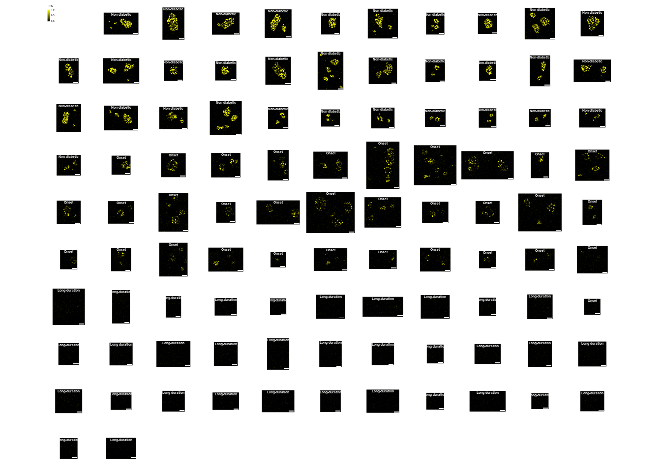
# Save plot
plotPixels(image = images[cur_order],
          colour_by = "PIN",
          scale_bar = list(length = 100,
                           label = "",
                           colour = "white"),
          colour = list(PIN = c("black", "yellow")),
          legend = list(margin = 100,
                        colour_by.title.cex = 8,
                        colour_by.labels.cex = 4),
          image_title = list(text = cur_meta$stage,
                             colour = "white",
                             cex = 3),
          save_plot = list(filename = "docs/final_figures/supplements/Fig_S2.png"))
Here, we see the progressive decline in beta cell fractions. The images are ordered based on T1D stage: Non-diabetic, Onset and Long-Duration, as expected. We further see an increased morphological irregularity in Long-Duration islets.
sessionInfo()R version 4.0.3 (2020-10-10)
Platform: x86_64-pc-linux-gnu (64-bit)
Running under: Ubuntu 20.04.1 LTS
Matrix products: default
BLAS/LAPACK: /usr/lib/x86_64-linux-gnu/openblas-pthread/libopenblasp-r0.3.8.so
locale:
[1] LC_CTYPE=en_US.UTF-8 LC_NUMERIC=C
[3] LC_TIME=en_US.UTF-8 LC_COLLATE=en_US.UTF-8
[5] LC_MONETARY=en_US.UTF-8 LC_MESSAGES=C
[7] LC_PAPER=en_US.UTF-8 LC_NAME=C
[9] LC_ADDRESS=C LC_TELEPHONE=C
[11] LC_MEASUREMENT=en_US.UTF-8 LC_IDENTIFICATION=C
attached base packages:
[1] parallel stats4 stats graphics grDevices utils datasets
[8] methods base
other attached packages:
[1] dplyr_1.0.2 cytomapper_1.2.0
[3] SingleCellExperiment_1.12.0 SummarizedExperiment_1.20.0
[5] Biobase_2.50.0 GenomicRanges_1.42.0
[7] GenomeInfoDb_1.26.0 IRanges_2.24.0
[9] S4Vectors_0.28.0 BiocGenerics_0.36.0
[11] MatrixGenerics_1.2.0 matrixStats_0.57.0
[13] EBImage_4.32.0 workflowr_1.6.2
loaded via a namespace (and not attached):
[1] viridis_0.5.1 viridisLite_0.3.0 svgPanZoom_0.3.4
[4] shiny_1.5.0 sp_1.4-4 GenomeInfoDbData_1.2.4
[7] vipor_0.4.5 tiff_0.1-6 yaml_2.2.1
[10] gdtools_0.2.2 pillar_1.4.6 lattice_0.20-41
[13] glue_1.4.2 digest_0.6.27 RColorBrewer_1.1-2
[16] promises_1.1.1 XVector_0.30.0 colorspace_2.0-0
[19] htmltools_0.5.0 httpuv_1.5.4 Matrix_1.2-18
[22] pkgconfig_2.0.3 raster_3.4-5 zlibbioc_1.36.0
[25] purrr_0.3.4 xtable_1.8-4 fftwtools_0.9-9
[28] scales_1.1.1 svglite_1.2.3.2 whisker_0.4
[31] jpeg_0.1-8.1 later_1.1.0.1 git2r_0.27.1
[34] tibble_3.0.4 generics_0.1.0 ggplot2_3.3.2
[37] ellipsis_0.3.1 magrittr_2.0.1 crayon_1.3.4
[40] mime_0.9 evaluate_0.14 fs_1.5.0
[43] beeswarm_0.2.3 shinydashboard_0.7.1 tools_4.0.3
[46] lifecycle_0.2.0 stringr_1.4.0 munsell_0.5.0
[49] locfit_1.5-9.4 DelayedArray_0.16.0 compiler_4.0.3
[52] systemfonts_0.3.2 rlang_0.4.8 grid_4.0.3
[55] RCurl_1.98-1.2 rstudioapi_0.13 htmlwidgets_1.5.2
[58] bitops_1.0-6 rmarkdown_2.5 gtable_0.3.0
[61] codetools_0.2-18 abind_1.4-5 R6_2.5.0
[64] gridExtra_2.3 knitr_1.30 fastmap_1.0.1
[67] rprojroot_2.0.2 stringi_1.5.3 ggbeeswarm_0.6.0
[70] Rcpp_1.0.5 vctrs_0.3.5 png_0.1-7
[73] tidyselect_1.1.0 xfun_0.19