Visualization of imaging cytometry data in R
Nils Eling
Department for Quantitative Biomedicine, University of ZurichInstitute for Molecular Health Sciences, ETH Zurichnils.eling@dqbm.uzh.ch
Nicolas Damond
Department for Quantitative Biomedicine, University of ZurichInstitute for Molecular Health Sciences, ETH Zurichnicolas.damond@dqbm.uzh.ch
Tobias Hoch
Department for Quantitative Biomedicine, University of ZurichInstitute for Molecular Health Sciences, ETH Zurichtobias.hoch@dqbm.uzh.ch
9 June 2026
Source:vignettes/cytomapper.Rmd
cytomapper.RmdAbstract
Highly multiplexed imaging cytometry acquires the single-cell expression of selected proteins in a spatially-resolved fashion. These measurements can be visualized across multiple length-scales. First, pixel-level intensities represent the spatial distributions of feature expression with highest resolution. Second, after segmentation, expression values or cell-level metadata (e.g. cell-type information) can be visualized on segmented cell areas. This package contains functions for the visualization of multiplexed read-outs and cell-level information obtained by multiplexed imaging cytometry. The main functions of this package allow 1. the visualization of pixel-level information across multiple channels and 2. the display of cell-level information (expression and/or metadata) on segmentation masks.
Introduction
This vignette gives an introduction to displaying highly-multiplexed
imaging cytometry data with the cytomapper package. As an
example, these instructions display imaging mass cytometry (IMC) data.
However, other imaging cytometry approaches including multiplexed ion
beam imaging (MIBI) (Angelo et al. 2014),
tissue-based cyclic immunofluorescence (t-CyCIF) (Lin et al. 2018) and iterative indirect
immunofluorescence imaging (4i) (Gut et al.
2018), which produce pixel-level intensities and optionally
segmentation masks can be displayed using cytomapper.
IMC (Giesen et al. 2014) is a multiplexed imaging cytometry approach to measure spatial protein abundance. In IMC, tissue sections are stained with a mix of around 40 metal-conjugated antibodies prior to laser ablation with resolution. The ablated material is transferred to a mass cytometer for time-of-flight detection of the metal ions [Giesen et al. (2014)](Mavropoulos et al., n.d.). In that way, hundreds of images (usually with an image size of around 1mm x 1mm) can be generated in a reasonable amount of time (Damond et al. 2019).
Raw IMC data are computationally processed using a segmentation pipeline (available at https://github.com/BodenmillerGroup/ImcSegmentationPipeline). This pipeline produces image stacks containing the raw pixel values for up to 40 channels, segmentation masks containing the segmented cells, cell-level expression and metadata information as well as a number of image-level meta information.
Cell-level expression and metadata can be processed and read into a
SingleCellExperiment class object. For more information on
the SingleCellExperiment object and how to create it,
please see the SingleCellExperiment
package and the Orchestrating
Single-Cell Analysis with Bioconductor workflow. Furthermore, the
cytomapper package provides the measureObjects function that generates a
SingleCellExperiment based on segmentation masks and
multi-channel images.
The cytomapper package provides a new
CytoImageList class as a container for multiplexed images
or segmentation masks. For more information on this class, refer to the
CytoImageList section.
The main functions of this package include plotCells and
plotPixels. The plotCells function requires
the following object inputs to display cell-level information
(expression and metadata):
- a
SingleCellExperimentobject, which contains the cells’ counts and metadata - a
CytoImageListobject containing the segmentation masks
The plotPixels function requires the following object
inputs to display pixel-level expression information:
- a
CytoImageListobject containing the pixel-level information per channel - (optionally) a
SingleCellExperimentobject, which contains the cells’ counts and metadata - (optionally) a
CytoImageListobject containing the segmentation masks
Quick start
The following section provides a quick example highlighting the
functionality of cytomapper. For detailed information on
reading in the data, refer to the Reading in
data section. More information on the required data format is
provided in the Data formats section. In the
first step, we will read in the provided toy
dataset
The CytoImageList object containing pixel-level
intensities representing the ion counts for five proteins can be
displayed using the plotPixels function:
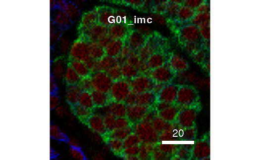
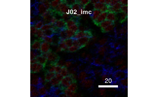
plotPixels(image = pancreasImages, colour_by = c("H3", "CD99", "CDH"))![]()
For more details on image normalization, cell outlining, and other pixel-level manipulations, refer to the Plotting pixel information section.
The CytoImageList object containing segmentation masks,
which represent cell areas on the image can be displayed using the
plotCells function. Only the segmentation masks are plotted
when no other parameters are specified.
To colour and/or outline segmentation masks, a
SingleCellExperiment, an img_id and
cell_id entry need to be specified:
plotCells(mask = pancreasMasks, object = pancreasSCE,
            cell_id = "CellNb", img_id = "ImageNb", colour_by = "CD99",
            outline_by = "CellType")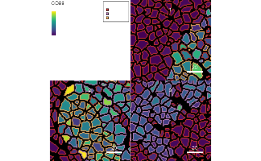
plotCells(mask = pancreasMasks, object = pancreasSCE,
            cell_id = "CellNb", img_id = "ImageNb",
            colour_by = "CellType")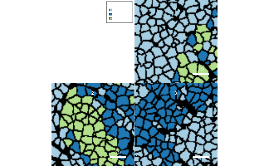
For more information on the data formats and requirements, refer to
the following section. More details on the plotCells
function are provided in the Plotting cell
information section. Also refer to the measureObjects function to generate a
SingleCellExperiment directly from the images.
Data formats
The cytomapper package combines objects of the SingleCellExperiment
class and the CytoImageList class (provided in
cytomapper) to visualize cell- and pixel-level
information.
In the main functions of the package, image refers to a
CytoImageList object containing one or multiple
multi-channel images where each channel represents the pixel-intensity
of one selected marker (proteins in the case of IMC). The entry
mask refers to a CytoImageList object
containing one or multiple segmentation masks. Segmentation masks are
defined as one-channel images containing integer values, which represent
the cells’ ids or 0 (background). Finally, the object entry
refers to a SingleCellExperiment class object that contains
cell-specific expression values (in the assay slots) and
cell-specific metadata in the colData slot.
To link information between the SingleCellExperiment and
CytoImageList objects, two slots need to be specified:
-
img_id: a single character indicating thecolData(in theSingleCellExperimentobject) andelementMetadata(in theCytoImageListobject) entry that contains the image identifiers. These image ids have to match between theSingleCellExperimentobject and theCytoImageListobject. -
cell_id: a single character indicating thecolDataentry that contains the cell identifiers. These should be integer values corresponding to pixel-values in the segmentation masks.
The img_id and cell_id entry in the
SingleCellExperiment object need to be accessible via:
head(colData(pancreasSCE)[,"ImageNb"])## [1] 1 1 1 1 1 1
head(colData(pancreasSCE)[,"CellNb"])## [1] 824 835 839 844 847 853The img_id entry in the CytoImageList
object need to be accessible via:
mcols(pancreasImages)[,"ImageNb"]## [1] 1 2 3
mcols(pancreasMasks)[,"ImageNb"]## [1] 1 2 3For more information on the CytoImageList class, please
refer to the section The CytoImageList
object. For more information on the
SingleCellExperiment object and how to create it, please
see the SingleCellExperiment
package and the Orchestrating
Single-Cell Analysis with Bioconductor workflow.
The provided toy dataset
For visualization purposes, the cytomapper package
provides a toy dataset containing 3 images of
x
dimensions (100 x 100 pixels). The dataset contains 362 segmented cells
and the expression values for 5 proteins: H3, CD99, PIN, CD8a, and CDH
It represents a small subset of the data presented in A
Map of Human Type 1 Diabetes Progression by Imaging Mass
Cytometry.
This dataset was generated using imaging mass cytometry (Giesen et al. 2014). Raw output files (in .mcd format) were processed using the IMC segmentation pipeline, which produces tiff-stacks containing the pixel-level information of all measured markers, segmentation masks that contain the cells’ object ids as well as cell- and image-specific measurements. Cell-specific measurements include the mean marker intensity per cell and per marker, the cells’ position and size measurements.
Pixel-level intensities for all 5 markers (5 channels) are stored in
the pancreasImages object. Entries to the
CytoImageList object and the rownames of
elementMetadata match: E34_imc, G01_imc, and J02_imc. The
elementMetadata slot (accesible via the
mcols() function) contains the image identifiers.
pancreasImages## CytoImageList containing 3 image(s)
## names(3): E34_imc G01_imc J02_imc
## Each image contains 5 channel(s)
## channelNames(5): H3 CD99 PIN CD8a CDH
mcols(pancreasImages)## DataFrame with 3 rows and 2 columns
## ImageName ImageNb
## <character> <integer>
## E34_imc E34 1
## G01_imc G01 2
## J02_imc J02 3
channelNames(pancreasImages)## [1] "H3" "CD99" "PIN" "CD8a" "CDH"
imageData(pancreasImages[[1]])[1:15,1:5,1]## [,1] [,2] [,3] [,4] [,5]
## [1,] 2.235787e+00 0.2537275 1.269632e+00 9.991982e-01 1.990020e+00
## [2,] 2.885528e+00 1.9900196 2.264642e+00 0.000000e+00 1.410924e+00
## [3,] 3.400943e+00 0.9950098 9.950098e-01 2.180066e+00 4.152935e-17
## [4,] 3.223832e+00 3.1750760 1.128341e+00 4.486604e+00 7.371460e-16
## [5,] 9.987666e-01 1.9900196 2.644036e-15 0.000000e+00 0.000000e+00
## [6,] 7.094598e-17 2.9412489 2.985029e+00 1.990020e+00 9.950098e-01
## [7,] 2.149031e-16 0.0000000 9.950098e-01 5.537247e-16 0.000000e+00
## [8,] 3.936259e+00 0.0000000 4.269442e-15 1.240777e+00 2.630806e+00
## [9,] 9.987666e-01 1.6437560 3.625816e+00 0.000000e+00 2.123351e+00
## [10,] 1.401616e-16 1.9900196 2.941249e+00 3.090500e+00 0.000000e+00
## [11,] 1.382069e+00 3.0258245 4.481710e-16 0.000000e+00 1.946239e+00
## [12,] 4.239594e+00 2.7720971 9.136457e-16 4.677541e+00 4.118345e+00
## [13,] 2.687521e+00 0.0000000 5.149176e+00 9.988809e-01 4.677541e+00
## [14,] 4.513364e+00 1.4666444 9.950098e-01 2.828813e+00 2.772097e+00
## [15,] 1.999239e+00 2.4616542 3.999584e+00 1.484527e+01 1.225784e+01The corresponding segmentation masks are stored in the
pancreasMasks object and can be read in from tiff images
containing the segmentation masks (see next section). Segmentation masks
are defined as one-channel images containing integer values, which
represent the cells’ ids or 0 (background).
pancreasMasks## CytoImageList containing 3 image(s)
## names(3): E34_mask G01_mask J02_mask
## Each image contains 1 channel
mcols(pancreasMasks)## DataFrame with 3 rows and 2 columns
## ImageName ImageNb
## <character> <integer>
## E34_mask E34 1
## G01_mask G01 2
## J02_mask J02 3
imageData(pancreasMasks[[1]])[1:15,1:5]## [,1] [,2] [,3] [,4] [,5]
## [1,] 824 824 824 824 0
## [2,] 824 824 824 824 0
## [3,] 824 824 824 824 0
## [4,] 824 824 824 824 824
## [5,] 824 824 824 824 824
## [6,] 824 824 824 824 824
## [7,] 824 824 824 824 824
## [8,] 824 824 824 824 824
## [9,] 824 824 824 824 824
## [10,] 824 824 824 824 0
## [11,] 824 824 824 0 0
## [12,] 824 824 0 0 0
## [13,] 0 0 0 0 864
## [14,] 0 0 0 864 864
## [15,] 0 864 864 864 864The IMC segmentation pipeline also generates cell-specific
measurements. The SingleCellExperiment class offers an
ideal container to store cell-specific expression counts together with
cell-specific metadata. For the toy dataset, cell-specific mean marker
intensities (counts) and arcsinh-transformed mean marker
intensities (exprs) are stored in the
assays(pancreasSCE) slot. All cell-specific metadata are
stored in the colData slot of the corresponding
SingleCellExperiment object: pancreasSCE. For
more information on the metadata, please refer to the
?pancreasSCE documentation. Of note: the cell-type labels
contained in the colData(pancreasSCE)$CellType slot are
arbitrary and only partly represent biologically relevant
cell-types.
pancreasSCE## class: SingleCellExperiment
## dim: 5 362
## metadata(0):
## assays(2): counts exprs
## rownames(5): H3 CD99 PIN CD8a CDH
## rowData names(4): MetalTag Target clean_Target frame
## colnames(362): E34_824 E34_835 ... J02_4190 J02_4209
## colData names(9): ImageName Pos_X ... MaskName Pattern
## reducedDimNames(0):
## mainExpName: NULL
## altExpNames(0):
names(colData(pancreasSCE))## [1] "ImageName" "Pos_X" "Pos_Y" "Area" "CellType" "ImageNb"
## [7] "CellNb" "MaskName" "Pattern"The pancreasSCE object also contains further information
on the measured proteins via the rowData(pancreasSCE) slot.
Furthermore, the pancreasSCE object contains the raw
expression counts per cell in the form of mean pixel value per cell and
protein (accessible via counts(pancreasSCE)). The
arcsinh-transformed (using a co-factor of 1) raw expression counts can
be obtained via assay(pancreasSCE, "exprs").
For more information on how to generate
SingleCellExperiment objects from count-based data, see Orchestrating
Single-Cell Analysis with Bioconductor.
Reading in data
The cytomapper package provides the
loadImages function to conveniently read images into a
CytoImageList object.
Load images
The loadImages function returns a
CytoImageList object containing the multi-channel images or
segmentation masks. Refer to the ?loadImages function to
see the full functionality.
As an example, we will read in multi-channel images and segmentation
masks provided by the cytomapper package.
# Read in masks
path.to.images <- system.file("extdata", package = "cytomapper")
all_masks <- loadImages(path.to.images, pattern = "_mask.tiff")
all_masks
## CytoImageList containing 3 image(s)
## names(3): E34_mask G01_mask J02_mask
## Each image contains 1 channel
# Read in images
all_stacks <- loadImages(path.to.images, pattern = "_imc.tiff")
all_stacks
## CytoImageList containing 3 image(s)
## names(3): E34_imc G01_imc J02_imc
## Each image contains 5 channel(s)Add metadata
To link images between the two CytoImageList objects and
the corresponding SingleCellExperiment object, the image
ids need to be added to the elementMetadata slot of the
CytoImageList objects. From the experimental setup, we know
that the image named ‘E34_imc’ has image id ‘1’, G01_imc has id ‘2’,
J02_imc has id ‘3’.
unique(pancreasSCE$ImageNb)## [1] 1 2 3Scale images
We can see that, in some cases, the pixel-values are not correctly scaled by the image encoding. The segmentation masks should only contain integer entries:
head(unique(as.numeric(all_masks[[1]])))## [1] 0.01257343 0.00000000 0.01318379 0.01310750 0.01287861 0.01280232The provided data was processed using CellProfiler (Carpenter et al. 2006). By default,
CellProfiler scales all pixel intensities between 0 and 1. This is done
by dividing each count by the maximum possible intensity value (see MeasureObjectIntensity
for more info). In the case of 16-bit encoding (where 0 is a valid
intensity), this scaling value is 2^16-1 = 65535.
Therefore, pixel-intensites need to be rescaled by this value. However,
this scaling value can change and different images can be scaled by
different factors. The user needs make sure to select the correct
factors in more complex cases.
The cytomapper package provides a
?scaleImages function. The user needs to manually scale
images to obtain the correct pixel-values. Here, we scale the
segmentation masks by the factor for 16-bit encoding:
2^16-1
all_masks <- scaleImages(all_masks, 2^16-1)
head(unique(as.numeric(all_masks[[1]])))
## [1] 824 0 864 859 844 839Alternatively, the as.is parameter can be set to
TRUE to attempt image scaling while reading in the
images:
all_masks_2 <- loadImages(path.to.images, pattern = "_mask.tiff", as.is = TRUE)
head(unique(as.numeric(all_masks_2[[1]])))
## [1] 824 0 864 859 844 839However, care needs to be taken and masks and images need to be checked if they are correctly imported.
For this toy dataset, the multi-channel images are not affected by
this scaling factor. The final all_masks object corresponds
to the pancreasMasks object provided by
cytomapper.
Add channel names
To access the correct images in the multi-channel
CytoImageList object, the user needs to set the correct
channel names. For this, the cytomapper package provides
the ?channelNames getter and setter function:
channelNames(all_stacks) <- c("H3", "CD99", "PIN", "CD8a", "CDH")The read-in data can now be used for visualization as explained in the Quick start section.
Generating the SingleCellExperiment object
Based on the processed segmentation masks and multi-channel images,
cytomapper can be used to measure cell-specific intensities
and morphological features. These features are stored in form of a
SingleCellExperiment object:
sce <- measureObjects(all_masks, all_stacks, img_id = "ImageNb")
sce
## class: SingleCellExperiment
## dim: 5 362
## metadata(0):
## assays(1): counts
## rownames(5): H3 CD99 PIN CD8a CDH
## rowData names(0):
## colnames: NULL
## colData names(8): ImageNb object_id ... m.majoraxis m.eccentricity
## reducedDimNames(0):
## mainExpName: NULL
## altExpNames(0):By default, the mean intensities per cell and channel are stored in
counts(sce) while all other morphological features are
stored in colData(sce):
counts(sce)[1:5, 1:5]## [,1] [,2] [,3] [,4] [,5]
## H3 1.50068681 12.7160872 2.16352437 4.6660460 3.4569734
## CD99 1.30339721 0.7676006 2.48035219 1.4353548 0.8031506
## PIN 0.03636109 0.3255984 0.07762631 0.1730306 0.2478255
## CD8a 0.20264913 0.0000000 0.28294494 0.5511711 0.1217455
## CDH 11.42480015 3.8496665 19.80123812 13.1796503 11.7225806
colData(sce)## DataFrame with 362 rows and 8 columns
## ImageNb object_id s.area s.radius.mean m.cx m.cy
## <character> <numeric> <numeric> <numeric> <numeric> <numeric>
## 1 1 824 55 3.93042 6.21818 2.96364
## 2 1 835 9 1.67054 94.44444 1.22222
## 3 1 839 17 2.47994 46.23529 1.70588
## 4 1 844 13 2.31966 33.92308 1.30769
## 5 1 847 87 4.92717 83.41379 4.66667
## ... ... ... ... ... ... ...
## 358 3 4165 10 1.34998 35.3000 99.0000
## 359 3 4167 34 3.09718 52.0882 98.7647
## 360 3 4173 1 0.00000 1.0000 100.0000
## 361 3 4190 2 0.50000 21.5000 100.0000
## 362 3 4209 12 1.60132 79.5000 99.3333
## m.majoraxis m.eccentricity
## <numeric> <numeric>
## 1 12.17659 0.863513
## 2 8.28709 0.985034
## 3 10.59886 0.977839
## 4 11.03438 0.985930
## 5 13.14283 0.570827
## ... ... ...
## 358 4.08496 0.514302
## 359 11.07958 0.932569
## 360 0.00000 0.000000
## 361 2.00000 1.000000
## 362 5.53775 0.842701The CytoImageList object
The cytomapper package provides a new
CytoImageList class, which inherits from the SimpleList
class. Each entry to the CytoImageList object is an
Image class object defined in the EBImage
package. A CytoImageList object is restricted to the
following entries:
- all images need to have the same number of channels
- the order/naming of channels need to be the same across all images
- entries to the
CytoImageListobject need to be uniquely named - names of
CytoImageListobject can either beNULLor should not containNAor empty entries - only grayscale images are supported (see
?Imagefor more information) - channels names do not support duplicated entries
CytoImageList objects that contain masks should only
contain a single channel
The following paragraphs will explain further details on manipulating
CytoImageList objects
Accessors
All accessor functions defined for SimpleList also work
on CytoImageList class objects. Element-wise metadata — in
the case of the CytoImageList object these are
image-specific metadata — are saved in the elementMetadata
slot. This slot can be accessed via the mcols()
function:
mcols(pancreasImages)## DataFrame with 3 rows and 2 columns
## ImageName ImageNb
## <character> <integer>
## E34_imc E34 1
## G01_imc G01 2
## J02_imc J02 3
mcols(pancreasImages)$PatientID <- c("Patient1", "Patient2", "Patient3")
mcols(pancreasImages)
## DataFrame with 3 rows and 3 columns
## ImageName ImageNb PatientID
## <character> <integer> <character>
## E34_imc E34 1 Patient1
## G01_imc G01 2 Patient2
## J02_imc J02 3 Patient3Subsetting a CytoImageList object works similar to a
SimpleList object:
pancreasImages[1]## CytoImageList containing 1 image(s)
## names(1): E34_imc
## Each image contains 5 channel(s)
## channelNames(5): H3 CD99 PIN CD8a CDH
pancreasImages[[1]]## Image
## colorMode : Grayscale
## storage.mode : double
## dim : 100 100 5
## frames.total : 5
## frames.render: 5
##
## imageData(object)[1:5,1:6,1]
## [,1] [,2] [,3] [,4] [,5] [,6]
## [1,] 2.2357869 0.2537275 1.269632e+00 0.9991982 1.990020e+00 0.000000e+00
## [2,] 2.8855283 1.9900196 2.264642e+00 0.0000000 1.410924e+00 5.654589e-16
## [3,] 3.4009433 0.9950098 9.950098e-01 2.1800663 4.152935e-17 1.990020e+00
## [4,] 3.2238317 3.1750760 1.128341e+00 4.4866042 7.371460e-16 0.000000e+00
## [5,] 0.9987666 1.9900196 2.644036e-15 0.0000000 0.000000e+00 1.523360e+00However, to facilitate subsetting and making sure that entry names
are transfered between objects, the cytomapper package
provides a number of getter and setter functions:
Getting and setting images
Individual or multiple entries in a CytoImageList object
can be obtained or replaced using the getImages and
setImages functions, respectively.
cur_image <- getImages(pancreasImages, "E34_imc")
cur_image
## CytoImageList containing 1 image(s)
## names(1): E34_imc
## Each image contains 5 channel(s)
## channelNames(5): H3 CD99 PIN CD8a CDH
setImages(pancreasImages, "New_image") <- cur_image
pancreasImages
## CytoImageList containing 4 image(s)
## names(4): E34_imc G01_imc J02_imc New_image
## Each image contains 5 channel(s)
## channelNames(5): H3 CD99 PIN CD8a CDH
mcols(pancreasImages)## DataFrame with 4 rows and 3 columns
## ImageName ImageNb PatientID
## <character> <integer> <character>
## E34_imc E34 1 Patient1
## G01_imc G01 2 Patient2
## J02_imc J02 3 Patient3
## New_image E34 1 Patient1The setImages function ensures that names are transfered
from one to the other object along the assignment operator:
names(cur_image) <- "Replacement"
setImages(pancreasImages, 2) <- cur_image
pancreasImages
## CytoImageList containing 4 image(s)
## names(4): E34_imc Replacement J02_imc New_image
## Each image contains 5 channel(s)
## channelNames(5): H3 CD99 PIN CD8a CDH
mcols(pancreasImages)## DataFrame with 4 rows and 3 columns
## ImageName ImageNb PatientID
## <character> <integer> <character>
## E34_imc E34 1 Patient1
## Replacement E34 1 Patient1
## J02_imc J02 3 Patient3
## New_image E34 1 Patient1However, if the image to replace is called by name, only the image and associated metadata is replaced:
setImages(pancreasImages, "J02_imc") <- cur_image
pancreasImages
## CytoImageList containing 4 image(s)
## names(4): E34_imc Replacement J02_imc New_image
## Each image contains 5 channel(s)
## channelNames(5): H3 CD99 PIN CD8a CDH
mcols(pancreasImages)## DataFrame with 4 rows and 3 columns
## ImageName ImageNb PatientID
## <character> <integer> <character>
## E34_imc E34 1 Patient1
## Replacement E34 1 Patient1
## J02_imc E34 1 Patient1
## New_image E34 1 Patient1Images can be deleted by setting the entry to NULL:
setImages(pancreasImages, c("Replacement", "New_image")) <- NULL
pancreasImages
## CytoImageList containing 2 image(s)
## names(2): E34_imc J02_imc
## Each image contains 5 channel(s)
## channelNames(5): H3 CD99 PIN CD8a CDHOf note: for plotting, the entries in the
img_id slot in the CytoImageList objects have
to be unique.
Getting and setting channels
The cytomapper package also provides functions to obtain
and replace channels. This functionality is provided via the
getChannels and setChannels functions:
cur_channel <- getChannels(pancreasImages, "H3")
cur_channel
## CytoImageList containing 2 image(s)
## names(2): E34_imc J02_imc
## Each image contains 1 channel(s)
## channelNames(1): H3
channelNames(cur_channel) <- "New_H3"
setChannels(pancreasImages, 1) <- cur_channel
pancreasImages
## CytoImageList containing 2 image(s)
## names(2): E34_imc J02_imc
## Each image contains 5 channel(s)
## channelNames(5): New_H3 CD99 PIN CD8a CDHThe setChannels function does not allow combining and
adding new channels. For this task, the cytomapper package
provides the mergeChannels section in the next
paragraph.
Naming and merging channels
Channel names can be obtained and replaced using the
channelNames getter and setter function:
channelNames(pancreasImages)## [1] "New_H3" "CD99" "PIN" "CD8a" "CDH"
channelNames(pancreasImages) <- c("ch1", "ch2", "ch3", "ch4", "ch5")
pancreasImages
## CytoImageList containing 2 image(s)
## names(2): E34_imc J02_imc
## Each image contains 5 channel(s)
## channelNames(5): ch1 ch2 ch3 ch4 ch5Furthermore, channels can be merged using the
mergeChannels function:
cur_channels <- getChannels(pancreasImages, 1:2)
channelNames(cur_channels) <- c("new_ch1", "new_ch2")
pancreasImages <- mergeChannels(pancreasImages, cur_channels)
pancreasImages
## CytoImageList containing 2 image(s)
## names(2): E34_imc J02_imc
## Each image contains 7 channel(s)
## channelNames(7): ch1 ch2 ch3 ch4 ch5 new_ch1 new_ch2Looping
To perform custom operations on each individual entry to a
CytoImageList object, the S4Vectors
package provides the endoapply function. While the
lapply function returns a list object, the
endoapply function provides an object of the same class of
the input object.
This allows the user to apply all functions provided by the EBImage
package to individual entries within the CytoImageList
object:
data("pancreasImages")

# Performing a gaussian blur
pancreasImages <- endoapply(pancreasImages, gblur, sigma = 1)
Plotting pixel information
The cytomapper package provides the
plotPixels function to plot pixel-level intensities of
marker proteins. The function requires a CytoImageList
object containing a single or multiple multi-channel images. To colour
images based on channel name, the channelNames of the
object need to be set. Furthermore, to outline cells, a
CytoImageList object containing segmentation masks and a
SingleCellExperiment object containing cell-specific
metadata need to be provided.
By default, pixel values are coloured internally and scaled between
the minimum and maximum values across all displayed images. However, to
manipulate pixel values and to linearly scale values to a certain range,
the cytomapper package provides a function for image
normalization.
Normalization
The normalize function provided in the
cytomapper package internally calls the
normalize function of the EBImage
package. The main difference between the two functions is the option to
scale per image or globally in the cytomapper package (see
?'normalize,CytoImageList-method').
By default, the normalize function linearly scales the
images channel-wise across all images and returns values between 0 and 1
(or the chosen ft range):
A CytoImageList object can also be normalized
image-wise:
# Image-wise normalization
cur_images <- normalize(pancreasImages, separateImages = TRUE)
To clip the image range, the user can provide a clipping range for all channels.
# Percentage-based clipping range
cur_images <- normalize(pancreasImages)
cur_images <- normalize(cur_images, inputRange = c(0, 0.9))
plotPixels(cur_images, colour_by = c("H3", "CD99", "CDH"))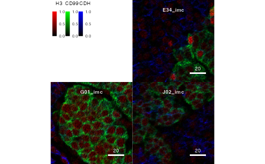
Alternatively, channel-specific clipping can be performed:
# Channel-wise clipping
cur_images <- normalize(pancreasImages,
                        inputRange = list(H3 = c(0, 70), CD99 = c(0, 100)))
For more information on the normalization functionality provided by
the cytomapper package, please refer to
?'normalize,CytoImageList-method'.
Colouring
The cytomapper package supports the visualization of up
to 6 channels and displays a combined image by setting the
colour_by parameter. See ?plotPixels for
examples.
Adjusting brightness, contrast and gamma
To enhance individual channels, the brightness (b), contrast (c) and
gamma (g) can be set channel-wise via the bcg parameter.
These parameters are set in form of a named list object.
Entry names need to correspond by channels specified in
colour_by. Each entry takes a numeric vector of length
three where the first entry represents the brightness value, the second
the contrast factor and the third the gamma factor. Internally, the
brightness value is added to each channel; each channel is multiplied by
the contrast factor and each channel is exponentiated by the gamma
factor.
data("pancreasImages")
# Increase contrast for the CD99 and CDH channel
plotPixels(pancreasImages,
            colour_by = c("H3", "CD99", "CDH"),
            bcg = list(CD99 = c(0,2,1),
CDH = c(0,2,1)))![]()
Outlining
The cells can be outlined when providing a CytoImageList
object containing the corresponding segmentation masks and a character
img_id indicating the name of the
elementMetadata slot that contains the image IDs.
The user can furthermore specify the metadata entry to outline cells
by. For this, a SingleCellExperiment object containing the
cell-specific metadata and a cell_id indicating the name of
the colData slot that contains the cell IDs need to be
provided:
plotPixels(pancreasImages, mask = pancreasMasks,
            object = pancreasSCE, img_id = "ImageNb",
            cell_id = "CellNb",
            colour_by = c("H3", "CD99", "CDH"),
outline_by = "CellType")![]()
Subsetting
The user can subset the images before calling the plotting functions:
cur_images <- getImages(pancreasImages, "J02_imc")
plotPixels(cur_images, colour_by = c("H3", "CD99", "CDH"))![]()
For further information on subsetting functionality, please refer to the Accessors section.
Adjusting the colour
The user can also customize the colours for selected features. The
colour parameter takes a named list in which
names correspond to the entries to colour_by. To colour
continous features such as expression or continous metadata entries
(e.g. cell area, see next section), at least two colours for
interpolation need to be provided. These colours are passed to the
colorRampPalette function for interpolation. For details,
please refer to the next Adjusting the
colour section
Plotting cell information
In the following sections, the plotCells function will
be introduced. This function displays cell-level information on
segmentation masks. It requires a CytoImageList object
containing segmentation masks in the form of single-channel images.
Furthermore, to colour and outline cells, a
SingleCellExperiment object containing cell-specific
expression counts and metadata needs to be provided.
By default, cell-specific expression values are coloured internally
and scaled marker-specifically between the minimum and maximum values
across the full SingleCellExperiment.
Colouring
Segmentation masks can be coloured based on the pixel-values averaged
across the area of each cell. In the SingleCellExperiment
object, these values can be obtained from the counts()
slot. To colour segmentation masks based on expression, the
rownames of the SingleCellExperiment must be
correctly named. The cytomapper package supports the
visualization of up to 6 channels and displays a combined image.
However, in the case of displaying expression on segmentation mask, the
user should not display too many features. See ?plotCells
for examples.
Changing the assay slot
To visualize differently transformed counts, the
plotCells function allows setting the
exprs_values parameter. In the toy dataset, the
assay(pancreasSCE, "exprs") slot contains the
arcsinh-transformed raw expression counts.
plotCells(pancreasMasks, object = pancreasSCE,
            img_id = "ImageNb", cell_id = "CellNb",
            colour_by = c("CD8a", "PIN"),
            exprs_values = "exprs")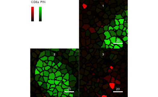
Outlining
The user can furthermore outline cells and specify the metadata entry
to outline cells by. See the previous Outlining
section and ?plotCells for examples.
Subsetting
Similar to the plotPixels function, the user can subset
the images before plotting. For an example, please see the previous Subsetting section and the Accessors section.
Adjusting the colour
The user can also customize the colours for selected features and
metadata. The colour parameter takes a named
list in which names correspond to the entries to
colour_by and/or outline_by. To colour
continous features such as expression or continous metadata entries
(e.g. cell area), at least two colours for interpolation need to be
provided. These colours are passed to the colorRampPalette
function for interpolation. To colour discrete entries, one colour per
entry needs to be specified in form of a named vector.
plotCells(pancreasMasks, object = pancreasSCE,
            img_id = "ImageNb", cell_id = "CellNb",
            colour_by = c("CD99", "CDH"),
            outline_by = "CellType",
            colour = list(CD99 = c("black", "red"),
                        CDH = c("black", "white"),
                        CellType = c(celltype_A = "blue",
                                    celltype_B = "green",
                                    celltype_C = "yellow")))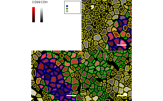
Customisation
The next sections explain different ways to customise the visual
output of the cytomapper package. To find more details on
additional parameters that can be set to customise the display, refer to
?'plotting-param'.
Subsetting the SingleCellExperiment object
The cytomapper package matches cells contained in the
SingleCellExperiment to objects contained in the
CytoImageList segmentation masks object via cell
identifiers. These are integer values, which are unique to each object
per image.
By matching these IDs, the user can subset the
SingleCellExperiment object and therefore only visualize
the cells retained in the object:
cur_sce <- pancreasSCE[,colData(pancreasSCE)$CellType == "celltype_A"]
plotCells(pancreasMasks, object = cur_sce,
            img_id = "ImageNb", cell_id = "CellNb",
            colour_by = "CellType",
            colour = list(CellType = c(celltype_A = "red")))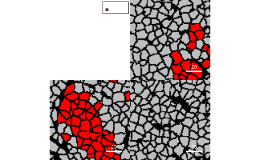
This feature is also helpful when visualising individual images. By
default, the legend will contain all metadata levels even those that are
not contained in the selected image. By subsetting the
SingleCellExperiment object to contain only the cells of
the selected image, the legend will only contain the metadata levels of
the selected cells.
Background and missing colour
The background of a segemntation mask is defined by the value
0. To change the background colour, the
background_colour parameter can be set. Furthermore, cells
that are not contained in the SingleCellExperiment object
can be coloured by setting missing_colour. For an example,
see figure @ref(fig:customization).
Scale bar and image title
Depending on the cells’ and background colour, the scale bar and
image title are not visible. To change the visual display of the scale
bar, a named list can be passed to the scale_bar parameter.
The list should contain one or multiple of the following entries:
length, label, cex,
lwidth, colour, position,
margin, frame. For a detailed explanation on
the individual entries, please refer to the scale_bar
section in ?'plotting-param'.
Of note: By default, the length of the scale bar is defined in number of pixels. Therefore, the user needs to know the length (e.g. in ) to label the scale bar correctly.
The image titles can be set using the image_title
parameter. Also here, the user needs to provide a named list with one or
multiple of follwing entries: text, position,
colour, margin, font,
cex. The entry to text needs to be a character
vector of the same length as the CytoImageList object.
Plotting of the scale bar and image title can be suppressed by
setting the scale_bar and image_title
parameters to NULL.
For an example, see figure @ref(fig:customization).
Legend
By default, the legend all all its contents are adjusted to the size
of the largest image in the CytoImageList object. However,
legend features can be altered by setting the legend
parameter. It takes a named list containing one or multiple of the
follwoing entries: colour_by.title.font,
colour_by.title.cex, colour_by.labels.cex,
colour_by.legend.cex, outline_by.title.font,
outline_by.title.cex, outline_by.labels.cex,
outline_by.legend.cex, margin. For detailed
explanation on the individual entries, please refer to the
legend parameter in ?'plotting-param'.
For an example, see figure @ref(fig:customization).
Setting the margin between images
To enhance the display of individual images, the
cytomapper package provides the margin
parameter.
The margin parameter takes a single numeric indicating
the gap (in pixels) between individual images.
For an example, see figure @ref(fig:customization).
Scale the feature counts
By default, features are scaled to the minimum and maximum per
channel. This behaviour facilitates visualization but does not allow the
user to visually compare absolute expression counts across channels. The
default behaviour can be suppressed by setting
scale = FALSE.
In this case, counts are linearly scaled to the minimum and maximum across all channels and across all displayed images.
For an example, see figure @ref(fig:customization).
Image interpolation
By default, colours are interpolated between pixels (see
?rasterImage for details). To suppress this default
behaviour, the user can set interpolate = FALSE.
Thick borders
By setting thick = TRUE, the thickness of the outline
border is increased. This setting can be useful to enhance the cell
borders on large images.
plotCells(pancreasMasks, object = pancreasSCE,
            img_id = "ImageNb", cell_id = "CellNb",
            colour_by = "CD99",
            outline_by = "CellType",
            background_colour = "white",
            missing_colour = "black",
            scale_bar = list(length = 30,
                            label = expression("30 " ~ mu * "m"),
                            cex = 2,
                            lwidth = 10,
                            colour = "cyan",
                            position = "bottomleft",
                            margin = c(5,5),
                            frame = 3),
            image_title = list(text = c("image_1", "image_2", "image_3"),
                            position = "topleft",
                            colour = "cyan",
                            margin = c(2,10),
                            font = 3,
                            cex = 2),
            legend = list(colour_by.title.font = 2,
                            colour_by.title.cex = 1.2,
                            colour_by.labels.cex = 0.7,
                            outline_by.legend.cex = 0.3,
                            margin = 10),
            margin = 2,
            thick = TRUE)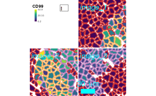
Plot customization example.
Returning plots and images
The user has the option to save the generated plots (see next
section) or to get the plots and/or coloured images returned. If
return_plot and/or return_images is set to
TRUE, cytomapper returns a list object with
one or two entries: plot and/or images.
The display parameter supports the entries
display = "all" (default), which displays images in a
grid-like fashion and display = "single", which display
images individually.
If the return_plot parameter is set to
TRUE, cytomapper internally calls the
recordPlot function and returns a plot object. The user can
additionally set display = "single" to get a list of plots
returned.
If the return_images parameter is set to
TRUE, cytomapper returns a
SimpleList object containing three-colour (red, green,
blue) Image objects.
cur_out <- plotPixels(pancreasImages, colour_by = c("H3", "CD99", "CDH"),
                return_plot = TRUE, return_images = TRUE,
                display = "single")

The returned plot objects now allows the plotting of individual images:
cur_out$plot$E34_imc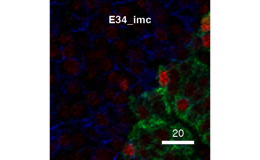
Furthermore, the user can directly plot the coloured images from the
returned SimpleList object:
plot(cur_out$images$G01_imc)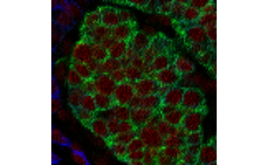
However, when plotting solely the coloured images, the image title and scale bar will be lost.
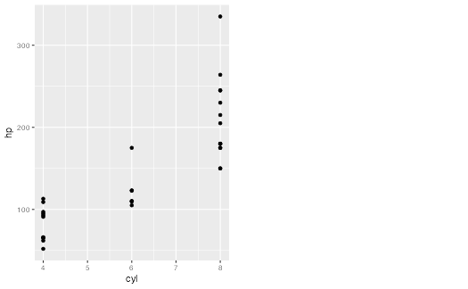
Integration with ggplot2 objects
The patchwork and
cowplot
R packages are popular frameworks to assemble full page figures
consisting of multiple sub-panels. This section will highlight how to
combine cytomapper plots and ggplot2 objects to create
larger figures.
library(cowplot)
library(ggplot2)

g1 <- ggplot(mtcars) + geom_point(aes(cyl, hp))
g2 <- plotCells(pancreasMasks, object = pancreasSCE,
            img_id = "ImageNb", cell_id = "CellNb",
            colour_by = "CellType", return_plot = TRUE)
Saving images
Finally, the user can save the plot by specifying
save_plot. The save_plot entry takes a list of
two entries: filename and scale. The
filename should be a character representing a valid file
name ending with .png, .tiff or
.jpeg. The scale entry controls the resolution
of the image (see ?"plotting-param" for help). Increasing
the scale parameter will increase the resolution of the final image.
When setting display = "single", the
cytomapper package will save individual images in
individual files. The filename will be altered to the form
filename_x.png where x is the position of the
image in the CytoImageList object or
legend.
Gating cells on images
The cytomapper package provides the
cytomapperShiny function to gate cells based on their
expression values and visualizes selected cells on their corresponing
images. This selection strategy can be useful if user-defined cell-type
labels should be generated for cell-type classification. For details,
please refer to the ?cytomapperShiny manual or the
Help button within the shiny application.
In brief, the cytomapperShiny function takes a
SingleCellExperiment and (optionally) either a
CytoImageList segmentation mask or a segmentation mask AND
a CytoImageList multi-channel image object as input. The
user needs to further provide an img_id and
cell_id entry (see above).
The user can specify the number of plots (maximal 12 plot, maximal 2
marker per plot), select the individual images (specified in the
img_id entry) and the different assay slots of
the SingleCellExperiment object. Furthermore, for each
plot, up to two markers can be selected for visualziation and gating.
Gating is performed in a hierarchical fashion meaning that only the
selected cells are displayed on the following plot. As an example: if
the user selects certain cells in Plot 1, the expression
values of only those cells are displayed in Plot 2 and so
on. If the user selects only one marker, the expression values are
displayed as violin/beeswarm plots; if two markers are specified,
expression values are displayed as scatter plots.
If the user provides a CytoImageList segmentation mask
object, the plotCells function is called internally to
visualize marker expression as well as the selected cells on the
segmentation mask. Pixel-level information is diplayed if the user
provides a CytoImageList multi-channel image object. In
this setting, the user also needs to provide a segmentation mask object
to outline the selected cells on the composite images.
As a final step, the user can download the selected cells in form of
a SingleCellExperiment object. Furthermore, the user can
specify a label for the current selection. The gates are stored in the
metadata(object) entry. Of note: the
metadata that was stored in the original object can be accessed via
metadata(object)$metadata.
Acknowledgements
We want to thank the Bodenmiller laboratory for feedback on the package and its functionality. Special thanks goes to Daniel Schulz and Jana Fischer for testing the package.
Contributions
Nicolas created the first version of cytomapper (named
IMCMapper). Nils and Nicolas implemented and maintain the
package. Nils and Tobias implemented and maintain the
cytomapperShiny function.
Session info
## R version 4.6.0 (2026-04-24)
## Platform: aarch64-apple-darwin23
## Running under: macOS Sequoia 15.7.7
##
## Matrix products: default
## BLAS:   /Library/Frameworks/R.framework/Versions/4.6/Resources/lib/libRblas.0.dylib
## LAPACK: /Library/Frameworks/R.framework/Versions/4.6/Resources/lib/libRlapack.dylib;  LAPACK version 3.12.1
##
## locale:
## [1] en_US.UTF-8/en_US.UTF-8/en_US.UTF-8/C/en_US.UTF-8/en_US.UTF-8
##
## time zone: UTC
## tzcode source: internal
##
## attached base packages:
## [1] stats4    stats     graphics  grDevices utils     datasets  methods
## [8] base
##
## other attached packages:
##  [1] ggplot2_4.0.3               cowplot_1.2.0
##  [3] cytomapper_1.25.0           SingleCellExperiment_1.34.0
##  [5] SummarizedExperiment_1.42.0 Biobase_2.72.0
##  [7] GenomicRanges_1.64.0        Seqinfo_1.2.0
##  [9] IRanges_2.46.0              S4Vectors_0.50.1
## [11] BiocGenerics_0.58.1         generics_0.1.4
## [13] MatrixGenerics_1.24.0       matrixStats_1.5.0
## [15] EBImage_4.54.0              BiocStyle_2.40.0
##
## loaded via a namespace (and not attached):
##  [1] bitops_1.0-9             gridExtra_2.3            rlang_1.2.0
##  [4] magrittr_2.0.5           svgPanZoom_0.3.4         shinydashboard_0.7.3
##  [7] otel_0.2.0               compiler_4.6.0           png_0.1-9
## [10] systemfonts_1.3.2        fftwtools_0.9-11         vctrs_0.7.3
## [13] pkgconfig_2.0.3          SpatialExperiment_1.22.0 fastmap_1.2.0
## [16] magick_2.9.1             XVector_0.52.0           labeling_0.4.3
## [19] promises_1.5.0           rmarkdown_2.31           ggbeeswarm_0.7.3
## [22] ragg_1.5.2               xfun_0.58                cachem_1.1.0
## [25] jsonlite_2.0.0           later_1.4.8              rhdf5filters_1.24.0
## [28] DelayedArray_0.38.2      Rhdf5lib_2.0.0           BiocParallel_1.46.0
## [31] jpeg_0.1-11              tiff_0.1-12              terra_1.9-27
## [34] parallel_4.6.0           R6_2.6.1                 bslib_0.11.0
## [37] RColorBrewer_1.1-3       jquerylib_0.1.4          Rcpp_1.1.1-1.1
## [40] bookdown_0.46            knitr_1.51               httpuv_1.6.17
## [43] Matrix_1.7-5             nnls_1.6                 tidyselect_1.2.1
## [46] abind_1.4-8              yaml_2.3.12              viridis_0.6.5
## [49] codetools_0.2-20         lattice_0.22-9           tibble_3.3.1
## [52] shiny_1.13.0             withr_3.0.2              S7_0.2.2
## [55] evaluate_1.0.5           desc_1.4.3               pillar_1.11.1
## [58] BiocManager_1.30.27      sp_2.2-1                 RCurl_1.98-1.19
## [61] scales_1.4.0             xtable_1.8-8             glue_1.8.1
## [64] tools_4.6.0              locfit_1.5-9.12          fs_2.1.0
## [67] rhdf5_2.56.0             grid_4.6.0               raster_3.6-32
## [70] beeswarm_0.4.0           HDF5Array_1.40.0         vipor_0.4.7
## [73] cli_3.6.6                textshaping_1.0.5        S4Arrays_1.12.0
## [76] viridisLite_0.4.3        svglite_2.2.2            dplyr_1.2.1
## [79] gtable_0.3.6             sass_0.4.10              digest_0.6.39
## [82] SparseArray_1.12.2       rjson_0.2.23             htmlwidgets_1.6.4
## [85] farver_2.1.2             htmltools_0.5.9          pkgdown_2.2.0
## [88] lifecycle_1.0.5          h5mread_1.4.0            mime_0.13