Detect the spatial context of each cell based on its neighborhood

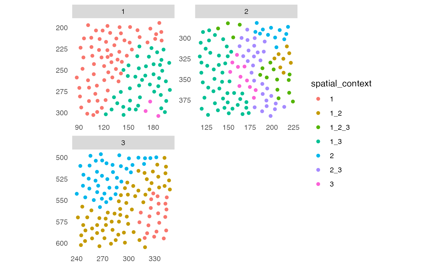
Function to detect the spatial context (SC) of each cell. Based on its sorted (high-to-low) cellular neighborhood (CN) fractions in a spatial interaction graph, the SC of each cell is assigned as the set of CNs that cumulatively exceed a user-defined fraction threshold.

The term was coined by Bhate S. et al., Tissue schematics map the specialization of immune tissue motifs and their appropriation by tumors, Cell Systems, 2022 and describes tissue regions in which distinct CNs may be interacting.

detectSpatialContext(
  object,
  entry = "aggregatedNeighbors",
  threshold = 0.9,
  name = "spatial_context"
)

Arguments

object: a SingleCellExperiment or SpatialExperiment object
entry: single character specifying the colData(object) entry containing the aggregateNeighbors DataFrame output. Defaults to "aggregatedNeighbors".
threshold: single numeric between 0 and 1 that specifies the fraction threshold for SC assignment. Defaults to 0.9.
name: single character specifying the name of the output saved in colData(object). Defaults to "spatial_context".

Value

returns an object of class(object) containing a new column entry to colData(object)[[name]]

Spatial context background

The function relies on CN fractions for each cell in a spatial interaction graph (originally a k-nearest neighbor (KNN) graph).

We can retrieve the CN fractions using the buildSpatialGraph and aggregateNeighbors functions.

The window size (k for KNN) for buildSpatialGraph should reflect a length scale on which biological signals can be exchanged and depends, among others, on cell density and tissue area. In view of their divergent functionality, we recommend to use a larger window size for SC (interaction between local processes) than for CN (local processes) detection.

Subsequently, the CN fractions are sorted from high-to-low and the SC of each cell is assigned the minimal combination of SCs that additively surpass a user-defined threshold. The default threshold of 0.9 aims to represent the dominant CNs, hence the most prevalent signals, in a given window.

For more details, please refer to: Bhate S. et al., Tissue schematics map the specialization of immune tissue motifs and their appropriation by tumors, Cell Systems, 2022.

References

Bhate S. et al., Tissue schematics map the specialization of immune tissue motifs and their appropriation by tumors, Cell Systems, 2022

Author

Lasse Meyer (lasse.meyer@uzh.ch)

Examples

set.seed(22)
library(cytomapper)
data(pancreasSCE)

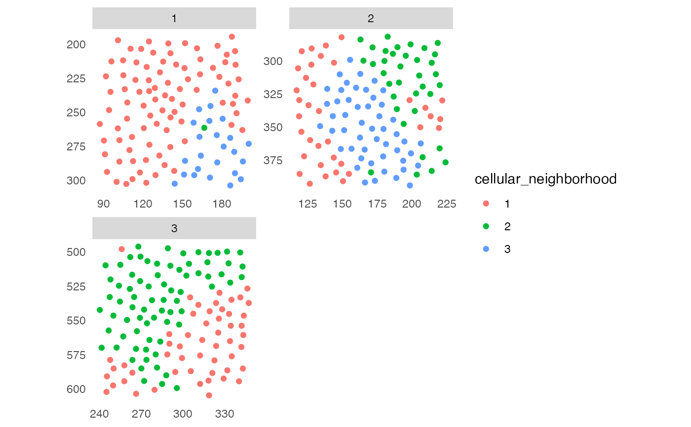
## 1. Cellular neighborhood (CN)
sce <- buildSpatialGraph(pancreasSCE, img_id = "ImageNb",
                        type = "knn",
                        name = "knn_cn_graph",
                        k = 5)
#> The returned object is ordered by the 'ImageNb' entry.

sce <- aggregateNeighbors(sce, colPairName = "knn_cn_graph",
                         aggregate_by = "metadata",
                         count_by = "CellType",
                         name = "aggregatedCellTypes")

cur_cluster <- kmeans(sce$aggregatedCellTypes, centers = 3)
sce$cellular_neighborhood <- factor(cur_cluster$cluster)

plotSpatial(sce, img_id = "ImageNb",
           colPairName = "knn_cn_graph",
           node_color_by = "cellular_neighborhood",
           scales = "free")


## 2. Spatial context (SC)
sce <- buildSpatialGraph(sce, img_id = "ImageNb",
                        type = "knn",
                        name = "knn_sc_graph",
                        k = 15)
#> The returned object is ordered by the 'ImageNb' entry.

sce <- aggregateNeighbors(sce, colPairName = "knn_sc_graph",
                         aggregate_by = "metadata",
                         count_by = "cellular_neighborhood",
                         name = "aggregatedNeighborhood")

# Detect spatial context
sce <- detectSpatialContext(sce, entry = "aggregatedNeighborhood",
                           threshold = 0.9)

plotSpatial(sce, img_id = "ImageNb",
           colPairName = "knn_sc_graph",
           node_color_by = "spatial_context",
           scales = "free")