Filter spatial contexts

Function to filter detected spatial contexts (SCs) based on a user-defined threshold for number of group entries and/or cells.

filterSpatialContext(
  object,
  entry = "spatial_context",
  group_by = "sample_id",
  group_threshold = NULL,
  cells_threshold = NULL,
  name = "spatial_context_filtered"
)

Arguments

object

a SingleCellExperiment or SpatialExperiment object

entry

a single character specifying the colData(object) entry containing the detectSpatialContext output. Defaults to "spatial_context".

group_by

a single character indicating the colData(object) entry by which SCs are grouped. This is usually the image or patient ID. Defaults to "sample_id".

group_threshold

a single numeric specifying the minimum number of group entries in which a SC is detected.

cells_threshold

a single numeric specifying the minimum total number of cells in a SC.

name

a single character specifying the name of the output saved in colData(object). Defaults to "spatial_context_filtered".

Value

returns an object of class(object) containing a new column entry to colData(object)[[name]] and a new data.frame entry to metadata(object)[["filterSpatialContext"]] containing the group and cell counts per SC.

References

Bhate S. et al., Tissue schematics map the specialization of immune tissue motifs and their appropriation by tumors, Cell Systems, 2022

See also

detectSpatialContext for the function to detect spatial contexts

plotSpatialContext for the function to plot spatial context graphs

Author

Lasse Meyer (lasse.meyer@uzh.ch)

Examples

set.seed(22)
library(cytomapper)
data(pancreasSCE)

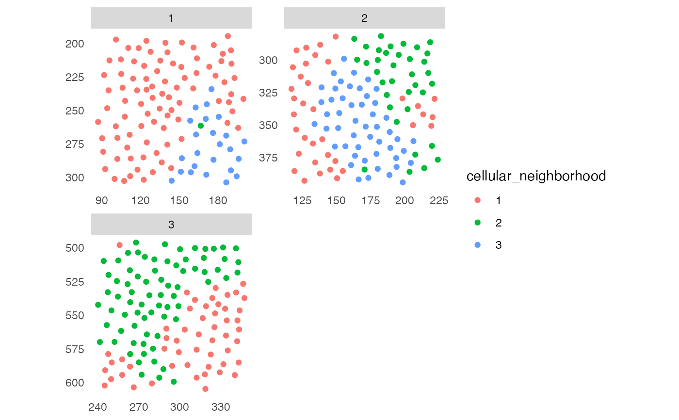
## 1. Cellular neighborhood (CN)
sce <- buildSpatialGraph(pancreasSCE, img_id = "ImageNb",
                        type = "knn",
                        name = "knn_cn_graph",
                        k = 5)
#> The returned object is ordered by the 'ImageNb' entry.

sce <- aggregateNeighbors(sce, colPairName = "knn_cn_graph",
                         aggregate_by = "metadata",
                         count_by = "CellType",
                         name = "aggregatedCellTypes")

cur_cluster <- kmeans(sce$aggregatedCellTypes, centers = 3)
sce$cellular_neighborhood <- factor(cur_cluster$cluster)

plotSpatial(sce, img_id = "ImageNb",
           colPairName = "knn_cn_graph",
           node_color_by = "cellular_neighborhood",
           scales = "free")


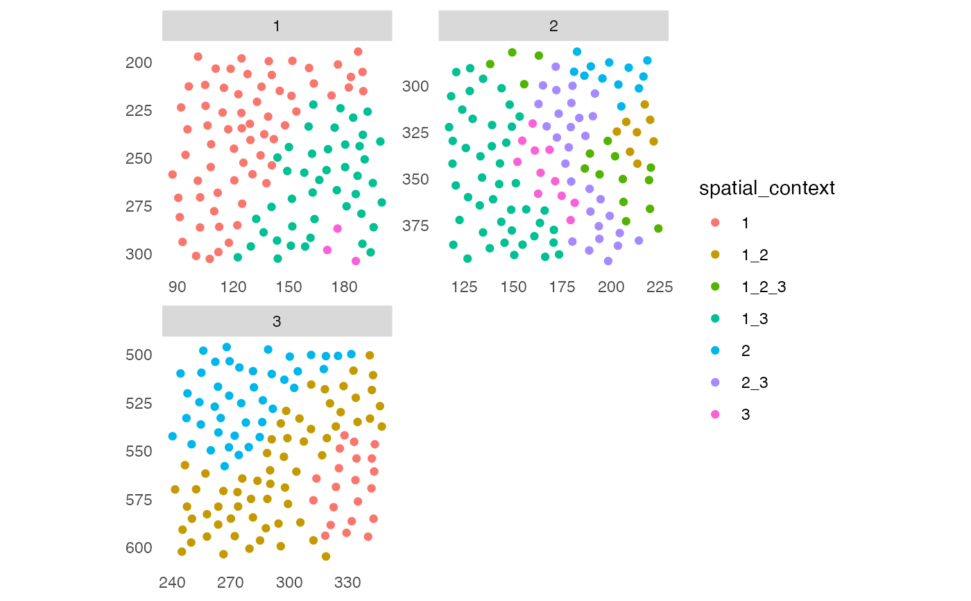
## 2. Spatial context (SC)
sce <- buildSpatialGraph(sce, img_id = "ImageNb",
                        type = "knn",
                        name = "knn_sc_graph",
                        k = 15)
#> The returned object is ordered by the 'ImageNb' entry.

sce <- aggregateNeighbors(sce, colPairName = "knn_sc_graph",
                         aggregate_by = "metadata",
                         count_by = "cellular_neighborhood",
                         name = "aggregatedNeighborhood")

# Detect spatial context
sce <- detectSpatialContext(sce, entry = "aggregatedNeighborhood",
                           threshold = 0.9)

plotSpatial(sce, img_id = "ImageNb",
           colPairName = "knn_sc_graph",
           node_color_by = "spatial_context",
           scales = "free")

            
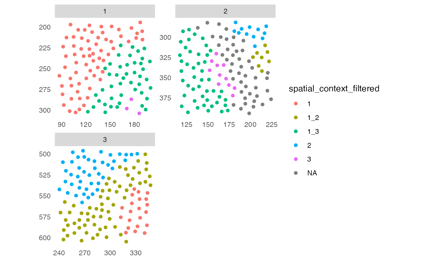
# Filter spatial context
# By group
sce <- filterSpatialContext(sce, group_by = "ImageNb", 
                            group_threshold = 2)

plotSpatial(sce, img_id = "ImageNb", 
            colPairName = "knn_sc_graph", 
            node_color_by = "spatial_context_filtered",
            scales = "free")


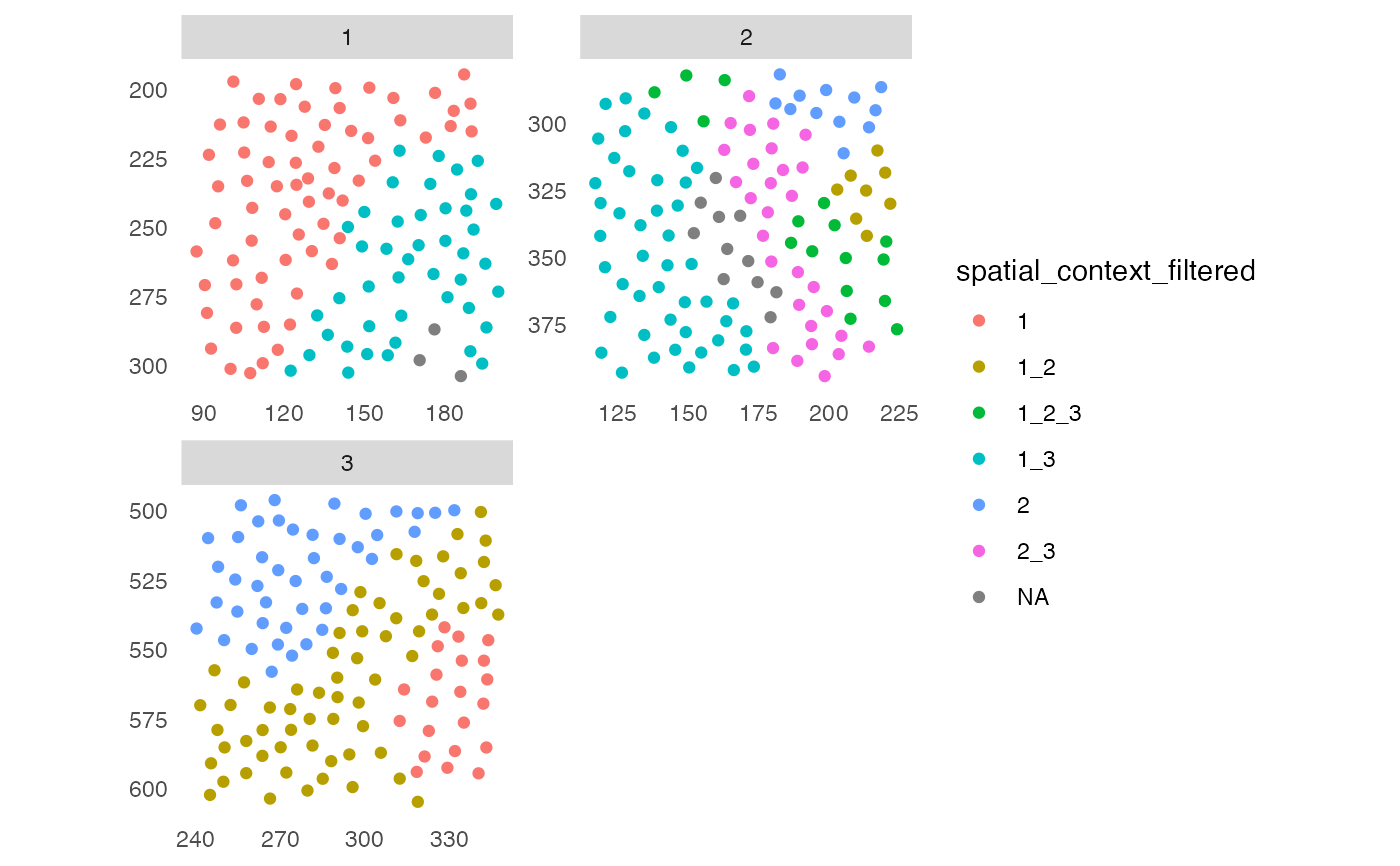
# By cells
sce <- filterSpatialContext(sce, group_by = "ImageNb", 
                            cells_threshold = 15)

plotSpatial(sce, img_id = "ImageNb", 
           colPairName = "knn_sc_graph", 
           node_color_by = "spatial_context_filtered",
           scales = "free")