Plot spatial context graph

Function to plot directed spatial context graphs based on symbolic edge-lists and vertex metadata, which operates on the cohort-level. The user can specify node, node_label and edge aesthetics.

plotSpatialContext(
  object,
  entry = "spatial_context",
  group_by = "sample_id",
  node_color_by = NULL,
  node_size_by = NULL,
  node_color_fix = NULL,
  node_size_fix = NULL,
  node_label_repel = TRUE,
  node_label_color_by = NULL,
  node_label_color_fix = NULL,
  draw_edges = TRUE,
  edge_color_fix = NULL,
  return_data = FALSE
)

Arguments

object

a SingleCellExperiment or SpatialExperiment object.

entry

single character specifying the colData(object) entry containing the detectSpatialContext output. Defaults to "spatial_context".

group_by

a single character indicating the colData(object) entry by which SCs are grouped. This is usually the image or patient ID. Defaults to "sample_id".

node_color_by

single character either NULL, "name","n_cells", "n_group" by which the nodes should be colored.

node_size_by

single character either NULL, "n_cells","n_group" by which the size of the nodes are defined.

node_color_fix

single character specifying the color of all nodes.

node_size_fix

single numeric specifying the size of all nodes.

node_label_repel

should nodes be labelled? Defaults to TRUE.

node_label_color_by

single character either NULL, "name","n_cells","n_group" by which the node labels should be colored.

node_label_color_fix

single character specifying the color of all node labels.

draw_edges

should edges be drawn between nodes? Defaults to TRUE.

edge_color_fix

single character specifying the color of all edges.

return_data

should the edge list and vertex metadata for graph construction be returned as a list of two data.frames?

Value

returns a ggplot object or a list of two data.frames.

References

Bhate S. et al., Tissue schematics map the specialization of immune tissue motifs and their appropriation by tumors, Cell Systems, 2022

See also

detectSpatialContext for the function to detect spatial contexts

filterSpatialContext for the function to filter spatial contexts

Author

Lasse Meyer (lasse.meyer@uzh.ch)

Examples

set.seed(22)
library(cytomapper)
data(pancreasSCE)

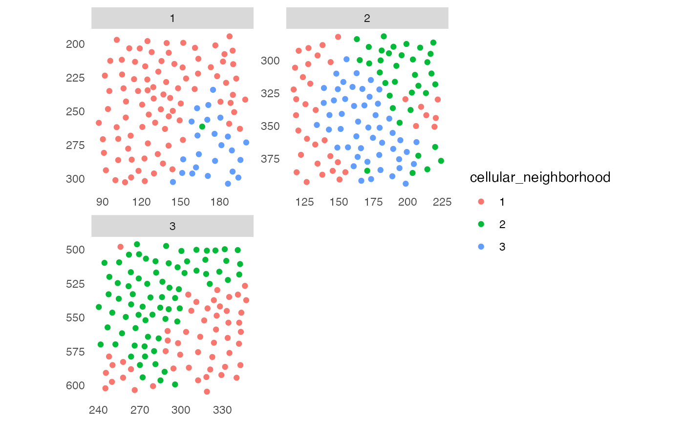
## 1. Cellular neighborhood (CN)
sce <- buildSpatialGraph(pancreasSCE, img_id = "ImageNb",
                        type = "knn",
                        name = "knn_cn_graph",
                        k = 5)
#> The returned object is ordered by the 'ImageNb' entry.

sce <- aggregateNeighbors(sce, colPairName = "knn_cn_graph",
                         aggregate_by = "metadata",
                         count_by = "CellType",
                         name = "aggregatedCellTypes")

cur_cluster <- kmeans(sce$aggregatedCellTypes, centers = 3)
sce$cellular_neighborhood <- factor(cur_cluster$cluster)

plotSpatial(sce, img_id = "ImageNb",
           colPairName = "knn_cn_graph",
           node_color_by = "cellular_neighborhood",
           scales = "free")


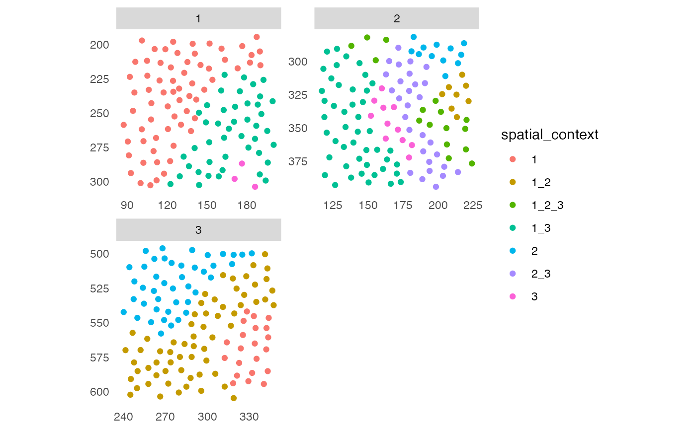
## 2. Spatial context (SC)
sce <- buildSpatialGraph(sce, img_id = "ImageNb",
                        type = "knn",
                        name = "knn_sc_graph",
                        k = 15)
#> The returned object is ordered by the 'ImageNb' entry.

sce <- aggregateNeighbors(sce, colPairName = "knn_sc_graph",
                         aggregate_by = "metadata",
                         count_by = "cellular_neighborhood",
                         name = "aggregatedNeighborhood")

# Detect spatial context
sce <- detectSpatialContext(sce, entry = "aggregatedNeighborhood",
                           threshold = 0.9)

plotSpatial(sce, img_id = "ImageNb",
           colPairName = "knn_sc_graph",
           node_color_by = "spatial_context",
           scales = "free")

            
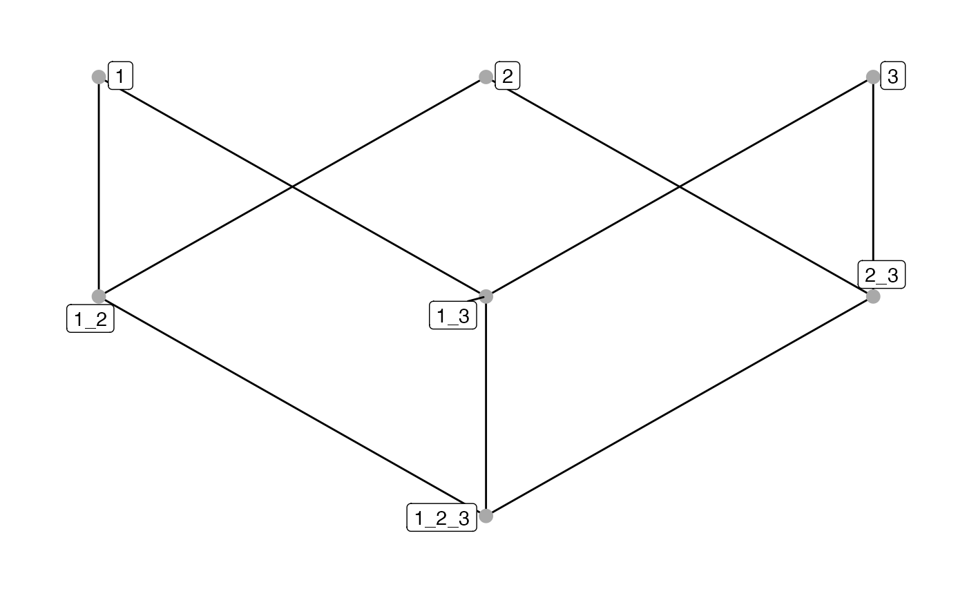
# Plot spatial context - default
plotSpatialContext(sce, group_by = "ImageNb")


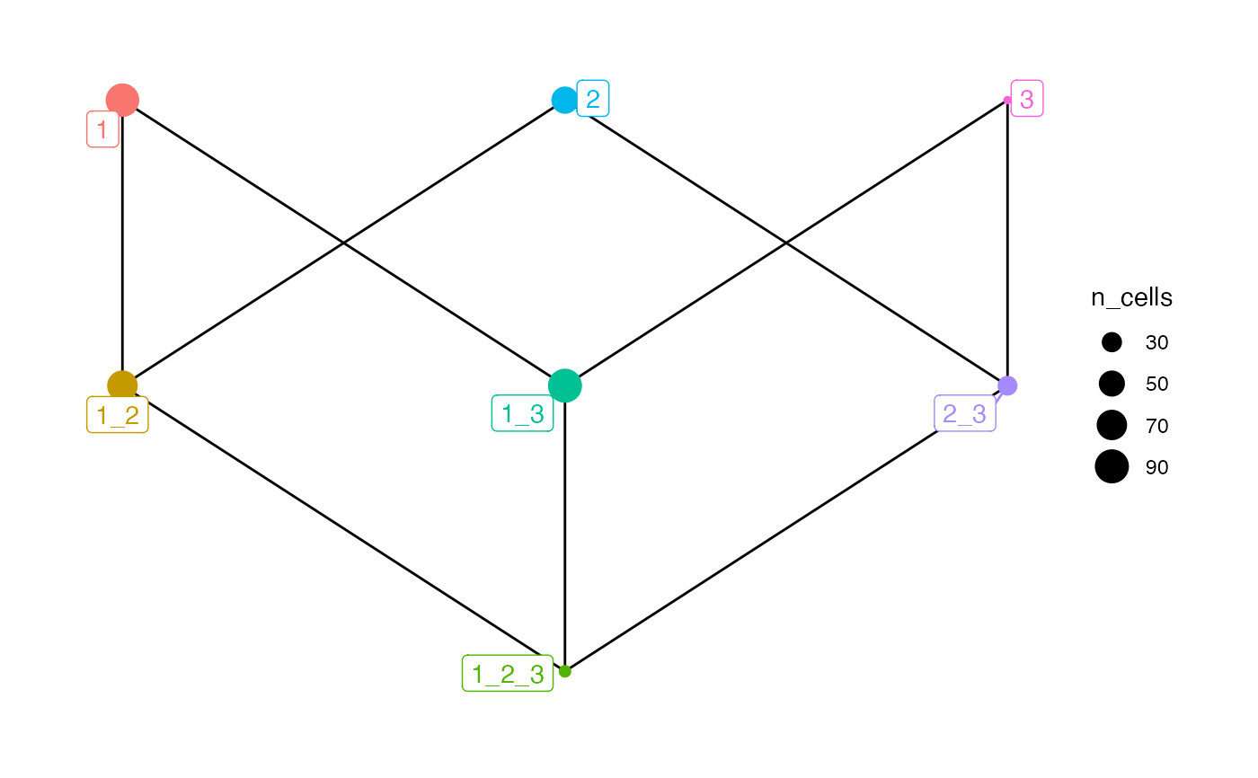
# Plot spatial context - adjust aesthetics
plotSpatialContext(sce, group_by = "ImageNb",
                   node_color_by = "name",
                   node_size_by = "n_cells",
                   node_label_color_by = "name")

                   
plotSpatialContext(sce, group_by = "ImageNb",
                   node_color_by = "n_cells",
                   node_size_by = "n_group")

                   
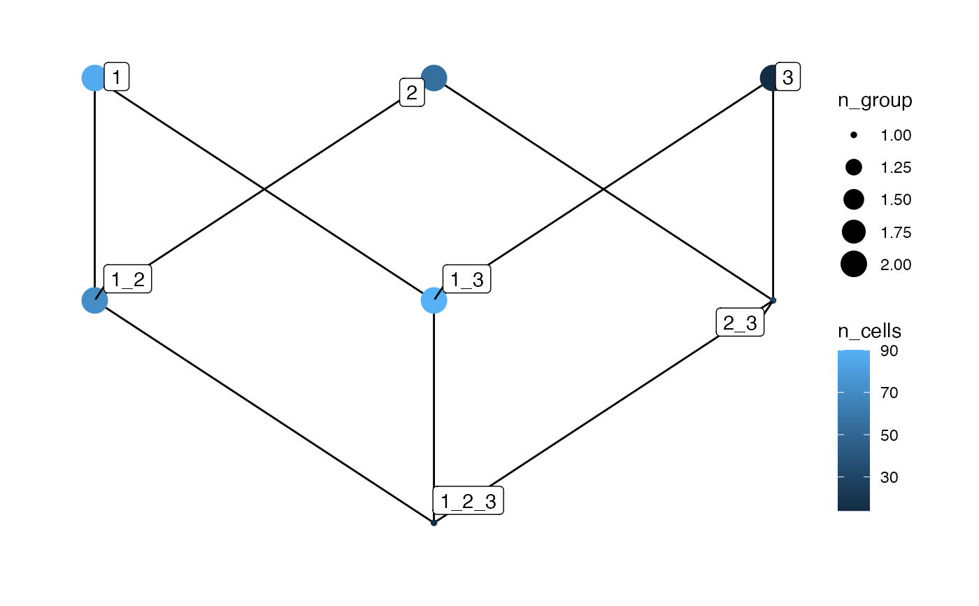# Plot spatial context - return data
plotSpatialContext(sce, group_by = "ImageNb",
                  return_data = TRUE)          
#> $edges
#>   from    to
#> 1    1   1_2
#> 2    1   1_3
#> 3  1_2 1_2_3
#> 4  1_3 1_2_3
#> 5    2   1_2
#> 6    2   2_3
#> 7  2_3 1_2_3
#> 8    3   1_3
#> 9    3   2_3
#> 
#> $vertices
#>   spatial_context n_cells n_group length
#> 1               1      87       2      1
#> 2             1_2      71       2      2
#> 3           1_2_3      16       1      3
#> 4             1_3      90       2      2
#> 5               2      55       2      1
#> 6             2_3      29       1      2
#> 7               3      14       2      1
#>